Slip distribution for different smoothing factors: (a) κ = 0 . 10, (b)

Download scientific diagram | Slip distribution for different smoothing factors: (a) κ = 0 . 10, (b) κ = 0 . 18, (c) κ = 0 . 30. We pick the second as the resultant model because of its good compatibility between weighted mis fi t and solution roughness. The numbers between the triangles in (a) indicate the segments. The white star denotes the epicenter from Harvard CMT solution.  from publication: 3-D coseismic displacement field of the 2005 Kashmir earthquake inferred from satellite radar imagery | Imagery, Imagery (Psychotherapy) and Earthquake | ResearchGate, the professional network for scientists.

3D coupled hydro-mechanical modeling of multi-decadal multi-zone saltwater disposal in layered and faulted poroelastic rocks and implications for seismicity: An example from the Midland Basin - ScienceDirect

Slip distribution for different smoothing factors: (a) κ = 0 . 10, (b)

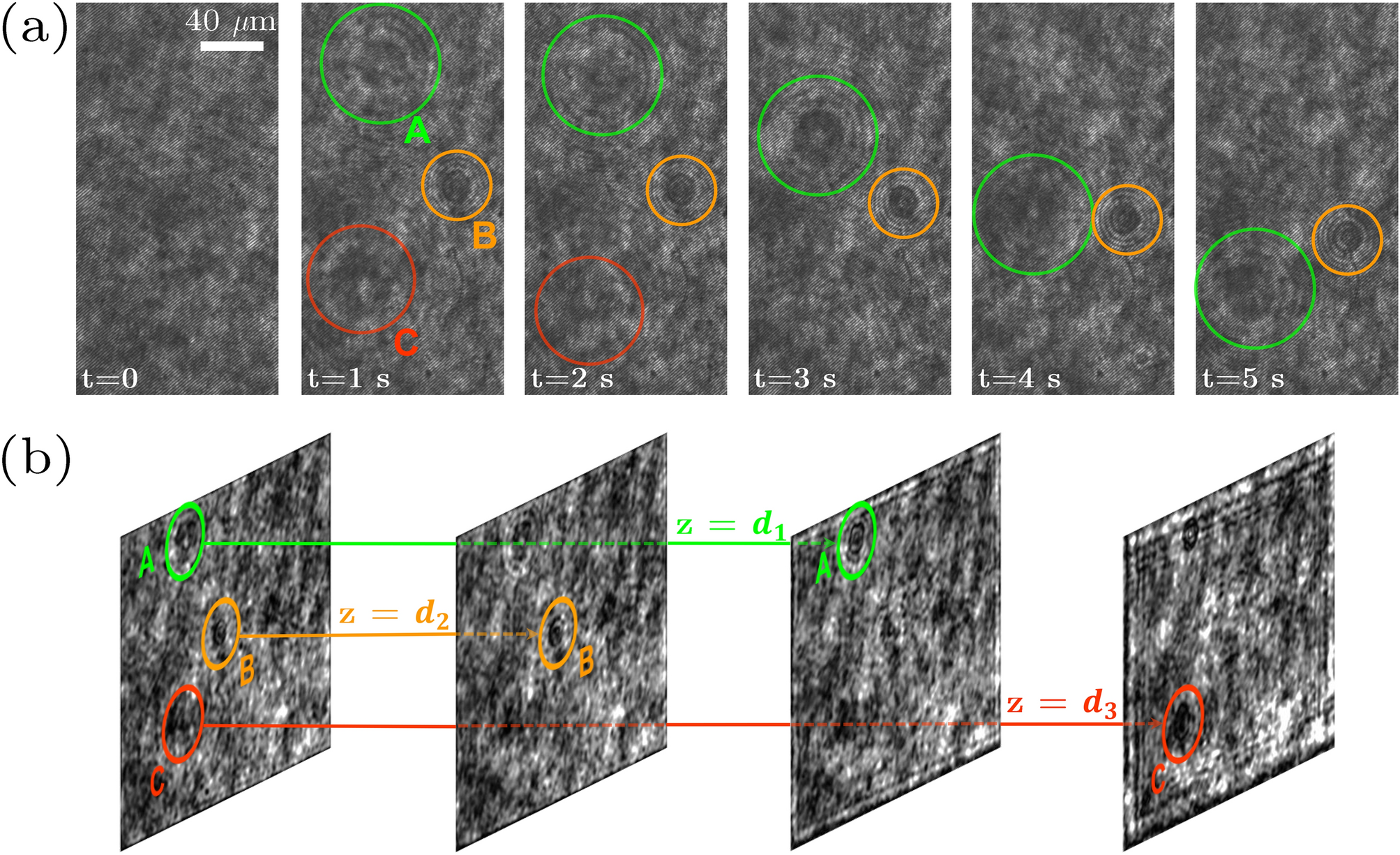
3D monitoring of the surface slippage effect on micro-particle sedimentation by digital holographic microscopy

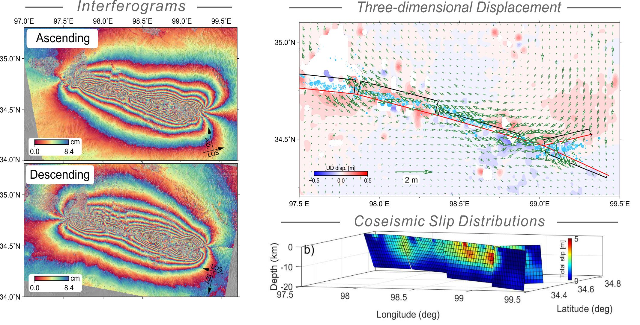
Finite fault slip models derived from InSAR observations. a, c are the

PDF) 3-D coseismic displacement field of the 2005 Kashmir earthquake inferred from satellite radar imagery

Analysis of coseismic slip distributions and stress variations of the 2019 Mw 6.4 and 7.1 earthquakes in Ridgecrest, California - ScienceDirect

Remote Sensing, Free Full-Text

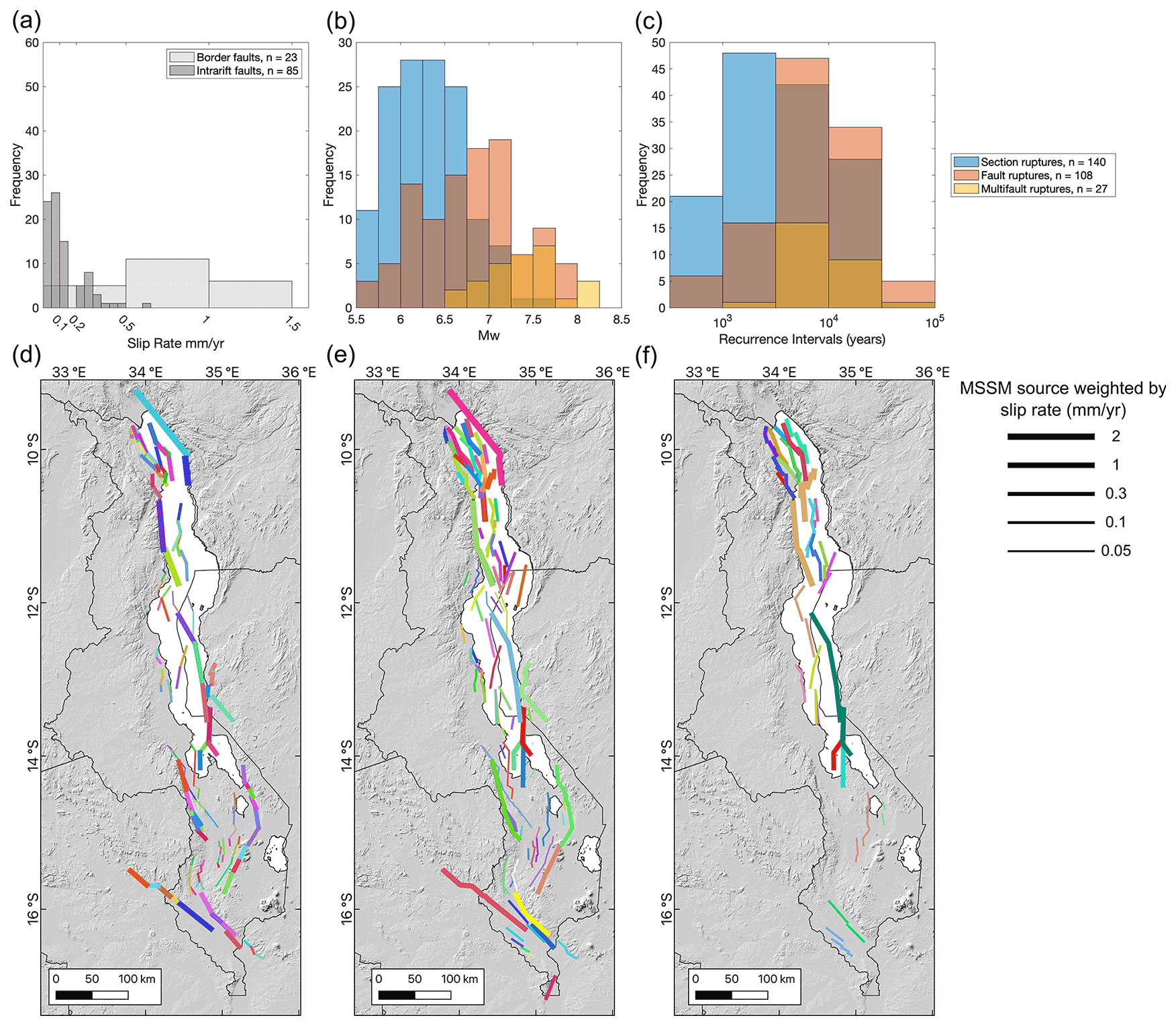
NHESS - Geologic and geodetic constraints on the magnitude and frequency of earthquakes along Malawi's active faults: the Malawi Seismogenic Source Model (MSSM)

Sensors, Free Full-Text

Remote Sensing, Free Full-Text